If you want to calculate biodiversity indices or perform community structure analysis (cluster analysis/NMDS), the best approach is to use the free statistical programming language 'R'. However, when I was a student, there was little documentation available, and writing code was a struggle. Variable assignment (definition) symbols, argument notation, and function naming all varied considerably from site to site, showing a great deal of inconsistency. Now, with progress in standardizing notation and the emergence of excellent generative AI like ChatGPT, the language has become much easier to read. Nevertheless, in this article, I would like to introduce an example of community structure analysis I performed using soil animal identification data.
- Example of soil animal analysis at a specific location
- How can I perform crowd structure analysis in R?
- How do I load data files?
- How can I calculate Shannon's diversity index and Simpson's diversity index using R?
- How do I plot NMDS using R?
- How do I perform cluster analysis using R?
- How can I perform indicator type analysis using R?
- References
Example of soil animal analysis at a specific location
The following are the identification results of soil animal samples extracted using the Tullgren method at four locations over two seasons. I was responsible for identifying all species except for beetles. We will use this data to calculate the biodiversity index and analyze the community structure.
The following is raw data; in reality, the analysis would involve aggregating the number of individuals of each entered species for each location and survey day, but this will be omitted here.
| Input type name | sex | population | Survey date | Survey location |
|---|---|---|---|---|
| Armored bead mite | 2 | May | A | |
| Flower mites | 2 | May | A | |
| Xylobates sp. | 21 | May | A | |
| Flat mite | 1 | May | A | |
| Asian giant mite | 1 | May | A | |
| Dwarf mites | 20 | May | A | |
| Cottony bead mites | 3 | May | A | |
| Family Scaridae sp. | 8 | May | A | |
| Yamato spider mites | 2 | May | A | |
| Stag beetle mites | 3 | May | A | |
| Himehesoirekodani | 2 | May | A | |
| Ghostly Tick | 1 | May | A | |
| Tokyo lily mite | 3 | May | A | |
| Veigaia sp. | 9 | May | A | |
| Parasitus sp. | 2 | May | A | |
| Family Tineidae sp. | 9 | May | A | |
| Podocinum sp. | 1 | May | A | |
| Pachylaelaps sp. | 1 | May | A | |
| Epicrius sp. | 6 | May | A | |
| Order Tinea, spp. | 24 | May | A | |
| Striped springtail | 1 | May | A | |
| Blue leafhopper springtail | 2 | May | A | |
| Small springtail | 7 | May | A | |
| Japanese white springtail | 1 | May | A | |
| Sacrum purpureus | 3 | May | A | |
| Yoshii forsom springtail | 1 | May | A | |
| Order Protaenia, sp. | 2 | May | A | |
| False ants | 6 | May | A | |
| Plum pine ant | 1 | May | A | |
| Teranishi's ant | 1 | May | A | |
| Centipede | 2 | May | A | |
| Takami's centipede | ♀ | 1 | May | A |
| Tajimagahara Hitofushimukade | ♀ | 1 | May | A |
| Monotarsobius sp. | ♂ | 1 | May | A |
| Fan millipede | 1 | May | A | |
| Mycosiidae sp. | 1 | May | A | |
| Variegated woodlouse | 1 | May | A | |
| Long-legged woodlice | 8 | May | A | |
| Family Tineidae sp. | 1 | May | A | |
| Dwarf mites | 2 | May | A | |
| Family Lumidae sp. | 10 | May | A | |
| Blue leafhopper springtail | 1 | May | B | |
| Striped springtail | 3 | May | B | |
| Small spiny springtail | 9 | May | B | |
| Sacrum purpureus | 15 | May | B | |
| Kotsunoari | 11 | May | B | |
| Soldier fly family sp. | 1 | May | B | |
| Centipede | 1 | May | B | |
| Flat mite | 1 | May | B | |
| Stag beetle mites | 1 | May | B | |
| Cottony bead mites | 2 | May | B | |
| Podocinum sp. | 1 | May | B | |
| Order Tinea, spp. | 3 | May | B | |
| Thrips (Amblyzolacera sp.). | 1 | May | B | |
| Ardisia japonica scale insect | 1 | May | B | |
| A species very similar to Watanabe's centipede | ♀♂ | 2 | May | B |
| Monotarsobius sp. | ♂ | 4 | May | B |
| Centipede | 3 | May | B | |
| Cottony bead mites | 23 | May | B | |
| Family Scaridae sp. | 2 | May | B | |
| Stag beetle mites | 7 | May | B | |
| Pale-colored umbilical cord mite | 1 | May | B | |
| Xylobates sp. | 5 | May | B | |
| Otafuku Daruma Mite | 1 | May | B | |
| Podocinum sp. | 2 | May | B | |
| Holaspina sp. | 4 | May | B | |
| Pachylaelaps sp. | ♂ | 4 | May | B |
| Parasitus sp. | 1 | May | B | |
| Order Tinea, spp. | 47 | May | B | |
| Abrolophus sp. | 1 | May | B | |
| Flower mites | 1 | May | C | |
| Armored bead mite | 1 | May | C | |
| Cottony bead mites | 10 | May | C | |
| Xylobates sp. | 46 | May | C | |
| Pale-colored umbilical cord mite | 1 | May | C | |
| Alameirekodani | 1 | May | C | |
| Yamato spider mites | 3 | May | C | |
| Dwarf mites | 2 | May | C | |
| Beak mites | 1 | May | C | |
| The smooth-skinned mite (Tricholoma rhodopolium) | 1 | May | C | |
| Podocinum sp. | 3 | May | C | |
| Family Tineidae sp. | 5 | May | C | |
| Veigaia sp. | 1 | May | C | |
| *Holostaspella* genus sp. | 4 | May | C | |
| Holaspina sp. | 2 | May | C | |
| Order Tinea, spp. | 12 | May | C | |
| Order Mites sp. | 1 | May | C | |
| Order Protaenia, sp. | 2 | May | C | |
| Sacrum purpureus | 2 | May | C | |
| Blue leafhopper springtail | 4 | May | C | |
| Striped springtail | 3 | May | C | |
| Northern scale ant | 1 | May | C | |
| False ants | 16 | May | C | |
| Teranishi's ant | 1 | May | C | |
| Kotsunoari | 26 | May | C | |
| Lepidoptera sp. | 1 | May | C | |
| Variegated woodlouse | 5 | May | C | |
| Long-legged woodlice | 1 | May | C | |
| Musashikamukade | 1 | May | C | |
| Fan millipede | 2 | May | C | |
| Mycosiidae sp. | 2 | May | C | |
| Monotarsobius sp. | ♂ | 6 | May | C |
| A species very similar to *Sakayori* centipede. | ♂ | 1 | May | C |
| Bothropolys sp. | 1 | May | C | |
| Pheretima sp. | 1 | May | C | |
| Family Lumidae sp. | 1 | May | C | |
| Two-eyed springtail | 3 | May | D | |
| Sacrum purpureus | 2 | May | D | |
| Japanese white springtail | 3 | May | D | |
| Family Stridae sp. | 4 | May | D | |
| Scale ants | 1 | May | D | |
| Kotsunoari | 29 | May | D | |
| Ameiro ant | 1 | May | D | |
| Soldier fly family sp. | 3 | May | D | |
| Family Tineidae sp. | 3 | May | D | |
| Family Tineidae sp. | 8 | May | D | |
| *Holostaspella* genus sp. | 4 | May | D | |
| Order Tinea, spp. | 10 | May | D | |
| Xylobates sp. | 11 | May | D | |
| Lasioseius sp. | ♂♀ | 2 | May | D |
| Southern spider mites | 6 | May | D | |
| Tokyo lily mite | 9 | May | D | |
| Cottony bead mites | 1 | May | D | |
| Himehesoirekodani | 1 | May | D | |
| Aphid mite | 1 | May | D | |
| Centipede | 1 | May | D | |
| Mycosiidae sp. | 9 | May | D | |
| Goshichinagasumukade | 1 | May | D | |
| Monotarsobius sp. | 1 | May | D | |
| Variegated woodlouse | 1 | May | D | |
| Long-legged woodlice | 9 | May | D | |
| Pheretima sp. | 1 | May | D | |
| Family Lumidae sp. | 1 | May | D | |
| Kotsunoari | 1 | August | A | |
| Ardisia japonica scale insect | 3 | August | A | |
| Mecistocephalus sp. | 1 | August | A | |
| Prolamnonyx sp. | 1 | August | A | |
| Variegated woodlouse | 3 | August | A | |
| Southern spider mites | 3 | August | A | |
| Flower mites | 1 | August | A | |
| Asian giant mite | 2 | August | A | |
| Two-spotted mites | 1 | August | A | |
| Ghostly Tick | 1 | August | A | |
| Stag beetle mites | 2 | August | A | |
| The smooth-skinned mite (Tricholoma rhodopolium) | 1 | August | A | |
| Dwarf mites | 1 | August | A | |
| Cottony bead mites | 1 | August | A | |
| Family Scaridae sp. | 1 | August | A | |
| Xylobates sp. | 1 | August | A | |
| Podocinum sp. | 2 | August | A | |
| Order Tinea, spp. | 4 | August | A | |
| Pheretima sp. | 1 | August | A | |
| Striped springtail | 1 | August | A | |
| Blue leafhopper springtail | 12 | August | A | |
| White springtail | 22 | August | A | |
| Small long springtail | 2 | August | A | |
| Pseudachorutes genus | 2 | August | A | |
| False ants | 4 | August | A | |
| Ameiro ant | 4 | August | A | |
| Northern scale ant | 3 | August | A | |
| Flat-tailed scale ants | 3 | August | A | |
| Kotsunoari | 4 | August | A | |
| Family Pentatomidae sp. larva | 1 | August | A | |
| Two-spotted mites | 1 | August | A | |
| Centipede | 3 | August | B | |
| Kirifuri Hitofushi Mukade | ♀ | 1 | August | B |
| A species very similar to Watanabe's centipede | ♂ | 1 | August | B |
| Eggplant centipede | ♂ | 1 | August | B |
| Monotarsobius sp. | 3 | August | B | |
| Pill bug | 1 | August | B | |
| Xylobates sp. | 1 | August | B | |
| Thick-legged mites | 10 | August | B | |
| Tokyo lily mite | 1 | August | B | |
| Holaspina sp. | 3 | August | B | |
| Podocinum sp. | 1 | August | B | |
| Order Tinea, spp. | 5 | August | B | |
| Japanese poppy | 1 | August | B | |
| Order Protaenia, sp. | 1 | August | B | |
| Striped springtail | 1 | August | B | |
| Himeforsom springtail | 49 | August | B | |
| Blue leafhopper springtail | 2 | August | B | |
| Two-eyed springtail | 2 | August | B | |
| Yoshii forsom springtail | 5 | August | B | |
| Small spiny springtail | 2 | August | B | |
| Sacrum purpureus | 1 | August | B | |
| Northern scale ant | 1 | August | B | |
| False ants | 1 | August | B | |
| Umematsu ant | 1 | August | B | |
| Kotsunoari | 69 | August | B | |
| Scale ants | 1 | August | B | |
| Elateridae sp. | 1 | August | B | |
| Thick-legged mites | 1 | August | B | |
| Ardisia japonica scale insect | 3 | August | C | |
| Centipede | 5 | August | C | |
| Monotarsobius sp. | ♂ | 4 | August | C |
| Mecistocephalus sp. | 2 | August | C | |
| Hirozu Gymnocalycium | 3 | August | C | |
| Variegated woodlouse | 6 | August | C | |
| Family Tineidae sp. | 6 | August | C | |
| *Holostaspella* genus sp. | 4 | August | C | |
| Order Tinea, spp. | 6 | August | C | |
| Xylobates sp. | 8 | August | C | |
| Flower mites | 1 | August | C | |
| Asian giant mite | 6 | August | C | |
| Aphid mite | 1 | August | C | |
| Order Protaenia, sp. | 8 | August | C | |
| Small long springtail | 13 | August | C | |
| Striped springtail | 2 | August | C | |
| Blue leafhopper springtail | 2 | August | C | |
| Sacrum purpureus | 2 | August | C | |
| Yellow-tailed ant | 1 | August | C | |
| Kotsunoari | 5 | August | C | |
| Northern scale ant | 2 | August | C | |
| Mealybug family sp. | 2 | August | D | |
| Kotsunoari | 1 | August | D | |
| Mycosiidae sp. | 1 | August | D | |
| Fan millipede | 3 | August | D | |
| genus *Haga millipede* | 2 | August | D | |
| Hirozu Gymnocalycium | 2 | August | D | |
| Monotarsobius sp. | 1 | August | D | |
| Variegated woodlouse | 9 | August | D | |
| Xylobates sp. | 1 | August | D | |
| Yamato spider mites | 4 | August | D | |
| Lasioseius sp. | 3 | August | D | |
| Cybaeus sp. | 2 | August | D | |
| Blue leafhopper springtail | 19 | August | D | |
| Yoshii forsom springtail | 2 | August | D | |
| Himeforsom springtail | 6 | August | D | |
| Small springtail | 2 | August | D | |
| Pseudachorutes sp. | 4 | August | D | |
| Order Protaenia, sp. | 1 | August | D | |
| Japanese subterranean termite | 19 | August | D | |
| Kotsunoari | 5 | August | D | |
| Elateridae sp. larva | 1 | August | D |
How can I perform crowd structure analysis in R?
The above data can be used to perform a crowd structure analysis in R. The complete code is provided below. This example uses R 4.3.2. Basic information is based on Takada (2018). Please also refer to Doi and Okamura (2011).
required_packages <- c("here", "vegan", "labdsv")

# パッケージがインストールされていなければインストールする
installed_packages <- rownames(installed.packages())
for (pkg in required_packages) {
  if (!pkg %in% installed_packages) {
    install.packages(pkg)
  }
}

# パッケージをロードする
lapply(required_packages, library, character.only = TRUE)

#ディレクトリの指定
getwd()
script_directory <- here("./土壌動物の室内分析と群集構造解析の例")
setwd(script_directory)

#分析データの読み込み
soil_data <- read.csv("土壌動物の個体数データ.csv", header = TRUE, row.names = 1, fileEncoding = "UTF-8")

# 生物多様性の計算
shannon_diversity <- diversity(soil_data, index = "shannon")
shannon_diversity

simpson_diversity <- diversity(soil_data, index = "simpson")
simpson_diversity

renyi(soil_data)

renyi_diversity <- exp(renyi(soil_data))
print(renyi_diversity)

# メタデータの多次元尺度構成法(MDS)解析
soil_data_matrix <- data.matrix(soil_data) # 行列に変換
mds_result <- metaMDS(soil_data_matrix, dist = "bray", autotransform = FALSE)
mds_result
ordipointlabel(mds_result, display = "sites", cex = 1, col = "black", pch = 16)


# クラスター解析
veg_dist <- vegdist(soil_data_matrix, method = "bray")
veg_dist

hierarchical_clustering <- hclust(veg_dist, method = "ward.D2")
hierarchical_clustering
plot(hierarchical_clustering, hang = -1)

# クラスタ数の評価
average_silhouette <- numeric(nrow(soil_data))
for (i in 2:(nrow(soil_data) - 1)) {
  silhouette_vals <- silhouette(cutree(hierarchical_clustering, k = i), veg_dist)
  average_silhouette[i] <- mean(silhouette_vals[, 3])
}
average_silhouette

# クラスタリングの結果
optimal_cluster <- cutree(hierarchical_clustering, k = which.max(average_silhouette))

# Silhouetteプロット
silhouette_vals <- silhouette(optimal_cluster, veg_dist)
rownames(silhouette_vals) <- row.names(soil_data)
plot(silhouette_vals)

# PAM法によるクラスタリングと重要な生物種の特定
pam_result <- pam(veg_dist, k = which.max(average_silhouette), diss = TRUE)
ind_val_analysis <- indval(soil_data, pam_result$clustering, numitr = 5000)
significant_groups <- ind_val_analysis$maxcls[ind_val_analysis$pval <= 0.05]
significant_species <- ind_val_analysis$indcls[ind_val_analysis$pval <= 0.05]
p_values <- ind_val_analysis$pval[ind_val_analysis$pval <= 0.05]
frequencies  0, 2, sum)[ind_val_analysis$pval <= 0.05]
significant_results <- data.frame(group = significant_groups, indval = significant_species, pvalue = p_values, freq = frequencies)
significant_results_summary <- significant_results[order(significant_results$group, -significant_results$indval), ]
significant_results_summary
How do I load data files?
First, install the packages we will be using. This step is unnecessary if you have already installed them.
required_packages <- c("here", "labdsv", "vegan")
install.packages(required_packages)install.packages(required_packages)Using the following code instead will skip packages that are already installed.
installed_packages <- rownames(installed.packages())
for (pkg in required_packages) {
  if (!pkg %in% installed_packages) {
    install.packages(pkg)
  }
}
While you can load them individually if you're not used to it, the code above allows you to reuse the package names as a vector when loading.
install.packages(here)
install.packages(labdsv)
install.packages(vegan)
Now, let's load the package.
lapply(required_packages, library, character.only = TRUE)Similarly, if you're not used to it, you can read them individually.
library(here)
library(labdsv)
library(vegan)
Next, specify the directory. You can specify the directory using an absolute path, but it's easier to specify the currently used workspace as the working directory.herePackagehere()I am using a function.here()Using this function is convenient because it allows you to share files on cloud storage like Google Drive, and the path remains valid even when you move files to a different PC.
However, it's important to note that the here() function retrieves the workspace path, so depending on your environment (in my case, VS Code), it may not specify the path above the currently open .R file. Therefore, I have to manually enter the path name one level up here. This is something that could be improved.
getwd()
script_directory <- here("./土壌動物の室内分析と群集構造解析の例")
setwd(script_directory)and,.csvThe file will be read. One thing to note is....csvThe file's character encoding must be UTF-8. This specification seems to have been added in a recent version, and I encountered problems when trying to run it with older R code. (This might be because I'm running it in VS Code.)
On PCs running Windows, creating a .csv file from an .xlsx file using Microsoft Excel or similar software will result in a .csv file with Shift-JIS (ANSI) character encoding.
Therefore, when saving a file using "Save As," choose the option that says "CSV UTF-8" instead of just "CSV." This is a very common mistake.
While it's technically possible to read.csv files using Shift-JIS encoding by setting the argument of read.csv() function to " fileEncoding = "Shift-JIS" ", Shift-JIS is an older standard, and UTF-8 is currently the backward-compatible character encoding. Therefore, using .csv files in their original encoding is not recommended.
In the following example, we've specified " fileEncoding = "UTF-8" just to be safe.
soil_data <- read.csv("土壌動物の個体数データ.csv", header = TRUE, row.names = 1, fileEncoding = "UTF-8")Data loading is now complete.
Common problems when reading .csv files include the orientation of columns and rows, and the presence or absence of labels.
The .csv file being imported in this example actually has the columns and rows reversed compared to the table above (the "Gender" row has also been removed). If you are using Microsoft Excel, you can easily reverse the rows and columns by right-clicking and selecting "Transpose" from the "Paste Options".
Also, if both the column and row have labels, specify " header = TRUE, row.names = 1 ".
How can I calculate Shannon's diversity index and Simpson's diversity index using R?
First, let's calculate the various biodiversity indices.
To calculate and view the Shannon diversity index, use the following code.
shannon_diversity <- diversity(soil_data, index = "shannon")
shannon_diversity
The following values were obtained this time.
| A(May) | B (May) | C(May) | D (May) | A (August) | B (August) | C (August) | D (August) |
|---|---|---|---|---|---|---|---|
| 3.081413 | 2.722761 | 2.739502 | 2.701395 | 2.820675 | 1.958188 | 2.829526 | 2.496044 |
To calculate and view the Simpson diversity index, use the following code.
simpson_diversity <- diversity(soil_data, index = "simpson")
simpson_diversity
The following values were obtained this time.
| A(May) | B (May) | C(May) | D (May) | A (August) | B (August) | C (August) | D (August) |
|---|---|---|---|---|---|---|---|
| 0.9319903 | 0.9061634 | 0.8824365 | 0.8974433 | 0.8955017 | 0.7420609 | 0.9303704 | 0.8756084 |
In all diversity indices, A (May) showed the highest diversity, while B (August) showed the lowest. Generally, one might expect insects to increase in number and population in August, but this was a surprising result.
How do I plot NMDS using R?
Next, let's perform Nonmetric Multidimensional Scaling (NMDS), a type of multivariate analysis. NMDS is a technique that arranges data in a low-dimensional space to reflect the similarity or distance between individual data points within a dataset.
In short, in this case, the closer the plots are in the diagram, the closer the biological community structure is.
To plot non-metric multidimensional scaling in R, use the following code:
soil_data_matrix <- data.matrix(soil_data) # 行列に変換
mds_result <- metaMDS(soil_data_matrix, dist = "bray", autotransform = FALSE)
mds_result
ordipointlabel(mds_result, display = "sites", cex = 1, col = "black", pch = 16)
As a result, the following figure was obtained.

The NMDS suggests seasonal influences on soil animal communities. While soil animals are generally considered less susceptible to seasonal changes, the increase in insects during the summer months likely played a role in this study. Site-specific influences are also evident, with site D showing significantly different results. Although there is no environmental information available for site D in this data, it is possible that the environment there undergoes significant seasonal changes. If quantitative environmental data were available, it would be possible to plot a more comprehensive evaluation of those influences.
How do I perform cluster analysis using R?
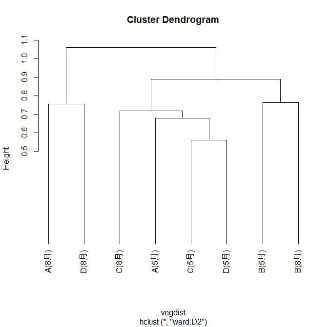
Next is cluster analysis. Cluster analysis is a statistical method that groups individual data points in a dataset based on similar characteristics or attributes, allowing us to understand the patterns and structures within the data. In this case, we will group the points in order of their closeness in terms of crowd structure. Cluster analysis and plotting can be performed using the following code.
This analysis uses the Bray-Curtis dissimilarity index.
veg_dist <- vegdist(soil_data_matrix, method = "bray")
veg_dist

hierarchical_clustering <- hclust(veg_dist, method = "ward.D2")
hierarchical_clustering
plot(hierarchical_clustering, hang = -1)
As a result, the following figure was obtained.
Silhouette analysis is performed using the following code. This method evaluates the results of clustering and measures how densely each data point is within its cluster. Silhouette analysis is one method for evaluating the validity of clustering and is useful in determining the number and shape of clusters.
In short, it's a handy tool that helps you avoid arbitrary group divisions and find meaningful criteria for dividing groups.
silhouette_vals <- silhouette(optimal_cluster, veg_dist)
rownames(silhouette_vals) <- row.names(soil_data)
plot(silhouette_vals)
As a result, the following diagram was obtained, and it was determined that dividing the data into two clusters (Cluster A (August) and Cluster D (August) and the other clusters) was optimal.
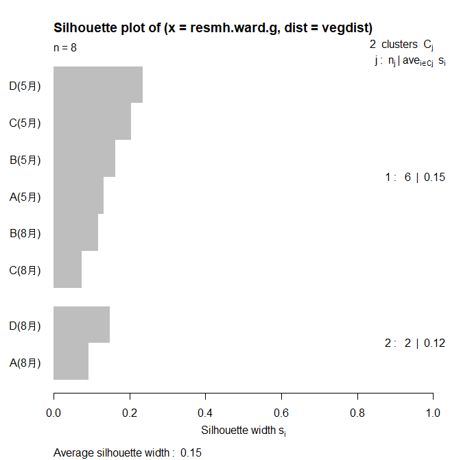
cutree() function allows you to determine which group each location belongs to.
| A(May) | B (May) | C(May) | D (May) | A (August) | B (August) | C (August) | D (August) |
|---|---|---|---|---|---|---|---|
| 1 | 1 | 1 | 1 | 2 | 1 | 1 | 2 |
In this particular cluster analysis example, there is very little information available about the ecology of each soil animal species, and environmental information such as the vegetation at the site is also lacking, making it difficult to draw conclusions. However, if this information is also included, a deeper analysis will be possible.
How can I perform indicator type analysis using R?
Finally, we perform an indicator species analysis based on cluster analysis. This can be done with the following code. Using the PAM method, we determine the optimal number of clusters, cluster the data, and identify important species for each cluster based on the clustering results. Then, we collect information on the identified important species (cluster, species, p-value, frequency of occurrence), summarize the important species for each cluster, and summarize the results.
pam_result <- pam(veg_dist, k = which.max(average_silhouette), diss = TRUE)
ind_val_analysis <- indval(soil_data, pam_result$clustering, numitr = 5000)
significant_groups <- ind_val_analysis$maxcls[ind_val_analysis$pval <= 0.05]
significant_species <- ind_val_analysis$indcls[ind_val_analysis$pval <= 0.05]
p_values <- ind_val_analysis$pval[ind_val_analysis$pval <= 0.05]
frequencies  0, 2, sum)[ind_val_analysis$pval <= 0.05]
significant_results <- data.frame(group = significant_groups, indval = significant_species, pvalue = p_values, freq = frequencies)
significant_results_summary <- significant_results[order(significant_results$group, -significant_results$indval), ]
significant_results_summary
Running this code will produce the following table.
| group | indval | pvalue | freq | |
|---|---|---|---|---|
| Sacrum purpureus | 1 | 1 | 0.0378 | 6 |
| Pseudachorutes sp. | 2 | 1 | 0.0374 | 2 |
This revealed that clusters A (August) and D (August) are indicated by the genus Pseudachorutes, while the other clusters are indicated by Pseudachorutes. Unfortunately, there is a lack of ecological information on these species as well, but a deeper analysis would be possible if we were to perform the analysis on species whose ecology is well known.
These analyses are possible for various biological communities, including insects, vertebrates, plants, aquatic organisms, and bacteria.
References
Doi, Hideyuki & Okamura, Hiroshi. (2011). Similarity and its applications for biological community analysis: Calculation, graphing, and testing of similarity using R. Journal of the Ecological Society of Japan, 61 (1), 3-20. https://doi.org/10.18960/seitai.61.1_3
Takada, Yoshitake. (2018). Analysis of community composition using R. Fisheries Research and Education Agency, Japan Sea Fisheries Research Institute. https://jsnfri.fra.affrc.go.jp/gunshu/index.html